Back to Article
Kaggle’s defaults
Download Notebook

Kaggle’s defaults

::: {#cell-2 .cell _uuid=‘8f2839f25d086af736a60e9eeb907d3b93b6e0e5’ _cell_guid=‘b1076dfc-b9ad-4769-8c92-a6c4dae69d19’ trusted=‘true’ quarto-private-1=‘{“key”:“execution”,“value”:{“iopub.status.busy”:“2026-06-19T11:25:44.713263Z”,“iopub.execute_input”:“2026-06-19T11:25:44.714087Z”,“iopub.status.idle”:“2026-06-19T11:25:45.430611Z”,“shell.execute_reply.started”:“2026-06-19T11:25:44.714037Z”,“shell.execute_reply”:“2026-06-19T11:25:45.429740Z”}}’ execution_count=1}

# This Python 3 environment comes with many helpful analytics libraries installed# It is defined by the kaggle/python Docker image: https://github.com/kaggle/docker-python# For example, here's several helpful packages to loadimport numpy as np # linear algebraimport pandas as pd # data processing, CSV file I/O (e.g. pd.read_csv)# Input data files are available in the read-only "../input/" directory# For example, running this (by clicking run or pressing Shift+Enter) will list all files under the input directoryimport osfor dirname, _, filenames in os.walk('/kaggle/input'):    for filename in filenames:        print(os.path.join(dirname, filename))# You can write up to 20GB to the current directory (/kaggle/working/) that gets preserved as output when you create a version using "Save & Run All" # You can also write temporary files to /kaggle/temp/, but they won't be saved outside of the current session# Use the kagglehub client library to attach Kaggle resources like competitions, datasets, and models to your session# Learn more about kagglehub: https://github.com/Kaggle/kagglehub/blob/main/README.mdimport kagglehub# kagglehub.dataset_download('<owner>/<dataset-slug>')
/kaggle/input/datasets/nikolazhuk/interp-emotions-prompts/prompts/joy.py
/kaggle/input/datasets/nikolazhuk/interp-emotions-prompts/prompts/neutral.py
/kaggle/input/datasets/nikolazhuk/interp-emotions-prompts/prompts/temporal.py

:::

Environment setup

In [2]:
# Tier-2 leaf libs pinned exactly. Tier-1 (torch/CUDA/python) inherited from the# pinned Kaggle image — do NOT pip-install torch here or you'll break the GPU.#%pip install -q "sae-lens==6.44.2" "transformer-lens==2.18.0" "sae-dashboard==0.7.2" "numpy==1.26.4"import osos.environ["PYTORCH_CUDA_ALLOC_CONF"] = "expandable_segments:True"os.environ["HF_HOME"] = "/tmp/hf"          # ephemeral scratch, not /contentfrom kaggle_secrets import UserSecretsClientos.environ["HF_TOKEN"] = UserSecretsClient().get_secret("HF_TOKEN")import torchtorch.set_grad_enabled(False)device = "cuda" if torch.cuda.is_available() else "cpu"# Fail fast if the leaf install disturbed tier-1:print("torch", torch.__version__, "| cuda", torch.version.cuda, "| device", device)assert device == "cuda", "GPU not visible — check Accelerator setting / install didn't swap torch"
torch 2.10.0+cu128 | cuda 12.8 | device cuda

Load model and SAE

In [3]:
from sae_lens import SAE, HookedSAETransformer# This avoids staging model in CPU RAM during loadmodel = HookedSAETransformer.from_pretrained(    "google/gemma-2-2b",    dtype=torch.float32,    device=device,    fold_ln=False,    center_writing_weights=False,    center_unembed=False,    move_to_device=True,)model.eval()print(f"n_layers={model.cfg.n_layers}, d_model={model.cfg.d_model}")sae, cfg_dict, sparsity = SAE.from_pretrained(    release="gemma-scope-2b-pt-res-canonical",    sae_id="layer_20/width_16k/canonical",    device=device)sae = sae.to(torch.bfloat16)allocated = torch.cuda.memory_allocated() / 1e9print(f"GPU allocated: {allocated:.1f}GB / 15GB")print(f"SAE d_sae: {sae.cfg.d_sae}, d_in: {sae.cfg.d_in}")print(sae.cfg.__dict__)
2026-06-19 11:25:59.067492: E external/local_xla/xla/stream_executor/cuda/cuda_fft.cc:467] Unable to register cuFFT factory: Attempting to register factory for plugin cuFFT when one has already been registered
WARNING: All log messages before absl::InitializeLog() is called are written to STDERR
E0000 00:00:1781868359.292954     155 cuda_dnn.cc:8579] Unable to register cuDNN factory: Attempting to register factory for plugin cuDNN when one has already been registered
E0000 00:00:1781868359.365838     155 cuda_blas.cc:1407] Unable to register cuBLAS factory: Attempting to register factory for plugin cuBLAS when one has already been registered
W0000 00:00:1781868359.901793     155 computation_placer.cc:177] computation placer already registered. Please check linkage and avoid linking the same target more than once.
W0000 00:00:1781868359.901833     155 computation_placer.cc:177] computation placer already registered. Please check linkage and avoid linking the same target more than once.
W0000 00:00:1781868359.901836     155 computation_placer.cc:177] computation placer already registered. Please check linkage and avoid linking the same target more than once.
W0000 00:00:1781868359.901838     155 computation_placer.cc:177] computation placer already registered. Please check linkage and avoid linking the same target more than once.
`torch_dtype` is deprecated! Use `dtype` instead!
Loaded pretrained model google/gemma-2-2b into HookedTransformer
n_layers=26, d_model=2304
GPU allocated: 15.2GB / 15GB
SAE d_sae: 16384, d_in: 2304
{'d_in': 2304, 'd_sae': 16384, 'dtype': 'bfloat16', 'device': 'cuda', 'apply_b_dec_to_input': False, 'normalize_activations': 'none', 'reshape_activations': 'none', 'metadata': SAEMetadata({'sae_lens_version': '6.44.2', 'sae_lens_training_version': None, 'model_name': 'gemma-2-2b', 'hook_name': 'blocks.20.hook_resid_post', 'hook_head_index': None, 'prepend_bos': True, 'dataset_path': 'monology/pile-uncopyrighted', 'context_size': 1024, 'neuronpedia_id': 'gemma-2-2b/20-gemmascope-res-16k'})}
/tmp/ipykernel_155/1363097899.py:17: DeprecationWarning: Unpacking SAE objects is deprecated. SAE.from_pretrained() now returns only the SAE object. Use SAE.from_pretrained_with_cfg_and_sparsity() to get the config dict and sparsity as well.
  sae, cfg_dict, sparsity = SAE.from_pretrained(

Reproduction of days-of-weeksFrom paper:NOT ALL LANGUAGE MODEL FEATURES AREONE-DIMENSIONALLY LINEAR: https://arxiv.org/pdf/2405.14860(residual PCA at layer 15)

In [4]:
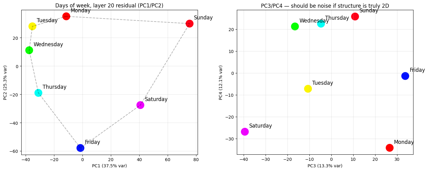
import numpy as npfrom sklearn.decomposition import PCAimport matplotlib.pyplot as pltDAYS = ["Monday", "Tuesday", "Wednesday", "Thursday", "Friday", "Saturday", "Sunday"]# Multiple templates per day to average out template-specific variationTEMPLATES = [    "Today is {}",    "She said it was {}",    "Yesterday was {}",    "I'll see you on {}",    "The meeting is on {}",    "He arrived on {}",    "The deadline was {}",    "School starts on {}",]LAYER = 20def last_token_resid(prompt: str, layer: int = LAYER) -> np.ndarray:    tokens = model.to_tokens(prompt)    _, cache = model.run_with_cache(        tokens,        names_filter=f"blocks.{layer}.hook_resid_post",        return_type=None,    )    return cache[f"blocks.{layer}.hook_resid_post"][0, -1].float().cpu().numpy()# (7, n_templates, d_model)day_vecs = np.stack([    np.stack([last_token_resid(t.format(d)) for t in TEMPLATES])    for d in DAYS])# Mean across templates → (7, d_model)day_means = day_vecs.mean(axis=1)# PCA to 4 components (we'll plot 1-2, but 3-4 are diagnostic)pca = PCA(n_components=4)day_pca = pca.fit_transform(day_means)# Plotfig, axes = plt.subplots(1, 2, figsize=(14, 7))# PC1 vs PC2ax = axes[0]ax.scatter(day_pca[:, 0], day_pca[:, 1], s=300, c=range(7), cmap="hsv")for i, day in enumerate(DAYS):    ax.annotate(day, (day_pca[i, 0], day_pca[i, 1]),                fontsize=12, xytext=(10, 10), textcoords="offset points")# Connect in calendar order, close the looploop = list(range(7)) + [0]ax.plot(day_pca[loop, 0], day_pca[loop, 1], "k--", alpha=0.3)ax.set_xlabel(f"PC1 ({pca.explained_variance_ratio_[0]:.1%} var)")ax.set_ylabel(f"PC2 ({pca.explained_variance_ratio_[1]:.1%} var)")ax.set_title(f"Days of week, layer {LAYER} residual (PC1/PC2)")ax.set_aspect("equal")ax.grid(alpha=0.3)# PC3 vs PC4 — should look like noise if days are truly 2Dax = axes[1]ax.scatter(day_pca[:, 2], day_pca[:, 3], s=300, c=range(7), cmap="hsv")for i, day in enumerate(DAYS):    ax.annotate(day, (day_pca[i, 2], day_pca[i, 3]),                fontsize=12, xytext=(10, 10), textcoords="offset points")ax.set_xlabel(f"PC3 ({pca.explained_variance_ratio_[2]:.1%} var)")ax.set_ylabel(f"PC4 ({pca.explained_variance_ratio_[3]:.1%} var)")ax.set_title("PC3/PC4 — should be noise if structure is truly 2D")ax.set_aspect("equal")ax.grid(alpha=0.3)plt.tight_layout()plt.show()print(f"Variance explained: {pca.explained_variance_ratio_}")print(f"Cumulative: {np.cumsum(pca.explained_variance_ratio_)}")

Variance explained: [0.37461206 0.25319353 0.132533   0.12052249]
Cumulative: [0.37461206 0.6278056  0.7603386  0.8808611 ]

Encoding residuals ->feature activations

In [5]:
def get_feature_acts(prompt: str, layer: int = 20):      tokens = model.to_tokens(prompt)      _, cache = model.run_with_cache(          tokens,          names_filter=f"blocks.{layer}.hook_resid_post",          return_type=None,      )      resid = cache[f"blocks.{layer}.hook_resid_post"].squeeze(  0).to(device).float()      feature_acts = sae.encode(resid)          # fp32 in → fp32 out      print("max act:", feature_acts.max().item(), "| nonzero:",  (feature_acts > 0).sum().item())      return feature_acts, model.to_str_tokens(prompt)

Days-of-wwek SAE decoder PCA

In [6]:
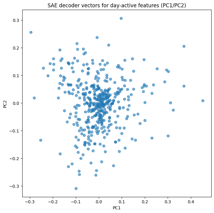
# Find SAE features that activate on day promptsdef features_active_on(prompt: str, threshold: float = 1.0):    acts, _ = get_feature_acts(prompt, layer=LAYER)    active = (acts[-1] > threshold).nonzero().squeeze(-1)    return active.cpu().numpy()# Union of features active on any day promptday_feature_set = set()for d in DAYS:    for t in TEMPLATES:        day_feature_set.update(features_active_on(t.format(d)).tolist())day_features = sorted(day_feature_set)print(f"Found {len(day_features)} candidate features active on day prompts")# Get their decoder vectors → (n_features, d_model)W_dec = sae.W_dec.float().cpu().numpy()  # (d_sae, d_model)day_decoders = W_dec[day_features]# PCA the decoder vectorspca_dec = PCA(n_components=4)dec_pca = pca_dec.fit_transform(day_decoders)# This plot won't directly show a 7-day circle — it shows clustering # structure across ALL features active on day prompts. The circle # emerges when you find the subcluster of ~7-14 features that # specifically co-activate by day.plt.figure(figsize=(8, 8))plt.scatter(dec_pca[:, 0], dec_pca[:, 1], alpha=0.6)plt.title("SAE decoder vectors for day-active features (PC1/PC2)")plt.xlabel("PC1"); plt.ylabel("PC2")plt.show()
max act: 2040.0 | nonzero: 7208
max act: 2040.0 | nonzero: 7313
max act: 2040.0 | nonzero: 7231
max act: 2040.0 | nonzero: 7475
max act: 2040.0 | nonzero: 7314
max act: 2040.0 | nonzero: 7234
max act: 2040.0 | nonzero: 7276
max act: 2040.0 | nonzero: 7285
max act: 2040.0 | nonzero: 7203
max act: 2040.0 | nonzero: 7308
max act: 2040.0 | nonzero: 7222
max act: 2040.0 | nonzero: 7475
max act: 2040.0 | nonzero: 7310
max act: 2040.0 | nonzero: 7239
max act: 2040.0 | nonzero: 7274
max act: 2040.0 | nonzero: 7282
max act: 2040.0 | nonzero: 7210
max act: 2040.0 | nonzero: 7308
max act: 2040.0 | nonzero: 7225
max act: 2040.0 | nonzero: 7475
max act: 2040.0 | nonzero: 7310
max act: 2040.0 | nonzero: 7238
max act: 2040.0 | nonzero: 7271
max act: 2040.0 | nonzero: 7280
max act: 2040.0 | nonzero: 7202
max act: 2040.0 | nonzero: 7314
max act: 2040.0 | nonzero: 7229
max act: 2040.0 | nonzero: 7475
max act: 2040.0 | nonzero: 7313
max act: 2040.0 | nonzero: 7238
max act: 2040.0 | nonzero: 7268
max act: 2040.0 | nonzero: 7283
max act: 2040.0 | nonzero: 7218
max act: 2040.0 | nonzero: 7316
max act: 2040.0 | nonzero: 7234
max act: 2040.0 | nonzero: 7468
max act: 2040.0 | nonzero: 7309
max act: 2040.0 | nonzero: 7233
max act: 2040.0 | nonzero: 7274
max act: 2040.0 | nonzero: 7284
max act: 2040.0 | nonzero: 7193
max act: 2040.0 | nonzero: 7307
max act: 2040.0 | nonzero: 7219
max act: 2040.0 | nonzero: 7470
max act: 2040.0 | nonzero: 7310
max act: 2040.0 | nonzero: 7233
max act: 2040.0 | nonzero: 7268
max act: 2040.0 | nonzero: 7276
max act: 2040.0 | nonzero: 7211
max act: 2040.0 | nonzero: 7312
max act: 2040.0 | nonzero: 7232
max act: 2040.0 | nonzero: 7470
max act: 2040.0 | nonzero: 7311
max act: 2040.0 | nonzero: 7235
max act: 2040.0 | nonzero: 7280
max act: 2040.0 | nonzero: 7281
Found 429 candidate features active on day prompts

Load temporal prompts: past, present, future, counterfactual and hypotheticalFrom Kaggle’s imported dataset

In [7]:
import sys, os, globhits = glob.glob("/kaggle/input/**/temporal.py", recursive=True)assert hits, "temporal.py not found under /kaggle/input — is the dataset attached?"sys.path.insert(0, os.path.dirname(hits[0]))from temporal import ALL_TEMPORAL_CATEGORIES

Geometry at 8, 14, 20, 25 layers

In [8]:
LAYERS = [8, 14, 20, 25]def last_token_resid(prompt: str, layer: int):    tokens = model.to_tokens(prompt)    _, cache = model.run_with_cache(        tokens,        names_filter=f"blocks.{layer}.hook_resid_post",        return_type=None,    )    return cache[f"blocks.{layer}.hook_resid_post"][0, -1].float()# Compute category means at every layerORDERED_CATS = ["past", "present", "future", "counterfactual", "hypothetical"]resid_means_by_layer = {}  # layer -> {cat: tensor(d_model,)}for L in LAYERS:    resid_means_by_layer[L] = {}    for cat in ORDERED_CATS:        vecs = [last_token_resid(p, L) for p in ALL_TEMPORAL_CATEGORIES[cat]]        resid_means_by_layer[L][cat] = torch.stack(vecs).mean(0)    print(f"Layer {L} done")
Layer 8 done
Layer 14 done
Layer 20 done
Layer 25 done
In [9]:
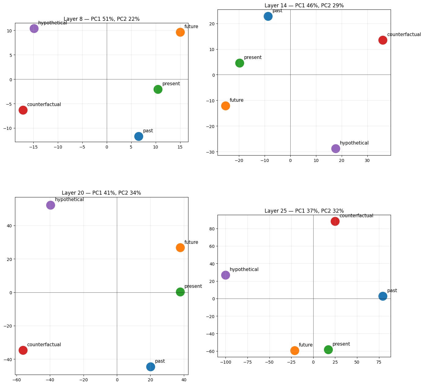
# Plot PCA grid: 2x2 layers, PC1/PC2 eachimport numpy as npfrom sklearn.decomposition import PCAimport matplotlib.pyplot as pltcolors = ["#1f77b4", "#2ca02c", "#ff7f0e", "#d62728", "#9467bd"]fig, axes = plt.subplots(2, 2, figsize=(14, 14))for ax, L in zip(axes.flat, LAYERS):    M = torch.stack([resid_means_by_layer[L][c] for c in ORDERED_CATS]).cpu().numpy()    M = M - M.mean(0, keepdims=True)    pca = PCA(n_components=2)    P = pca.fit_transform(M)    for i, cat in enumerate(ORDERED_CATS):        ax.scatter(P[i, 0], P[i, 1], s=400, c=colors[i])        ax.annotate(cat, (P[i, 0], P[i, 1]),                    fontsize=11, xytext=(10, 10), textcoords="offset points")    ax.set_title(f"Layer {L} — PC1 {pca.explained_variance_ratio_[0]:.0%}, "                 f"PC2 {pca.explained_variance_ratio_[1]:.0%}")    ax.axhline(0, color="k", lw=0.4); ax.axvline(0, color="k", lw=0.4)    ax.grid(alpha=0.3); ax.set_aspect("equal")plt.tight_layout()plt.show()

Temporal category means at layer 20

In [10]:
# === STEP 1: Compute category means (last-token aggregation) ===from temporal import ALL_TEMPORAL_CATEGORIEScategory_means_sae = {}  # category -> mean SAE activation vector (d_sae,)category_means_resid = {}  # category -> mean residual stream vector (d_model,)for cat_name, prompts in ALL_TEMPORAL_CATEGORIES.items():    sae_vecs = []    resid_vecs = []    for p in prompts:        # SAE features (uses your existing get_feature_acts)        acts, _ = get_feature_acts(p, layer=20)        sae_vecs.append(acts[-1])        # Raw residual (for the Engels-style PCA)        tokens = model.to_tokens(p)        _, cache = model.run_with_cache(            tokens, names_filter="blocks.20.hook_resid_post", return_type=None,        )        resid_vecs.append(cache["blocks.20.hook_resid_post"][0, -1].float())    category_means_sae[cat_name]   = torch.stack(sae_vecs).mean(0)    category_means_resid[cat_name] = torch.stack(resid_vecs).mean(0)    print(f"{cat_name:>15}: {len(prompts)} prompts processed")
max act: 2040.0 | nonzero: 7539
max act: 2040.0 | nonzero: 7409
max act: 2040.0 | nonzero: 7524
max act: 2040.0 | nonzero: 7504
max act: 2040.0 | nonzero: 7503
max act: 2040.0 | nonzero: 7528
max act: 2040.0 | nonzero: 7508
max act: 2040.0 | nonzero: 7520
max act: 2040.0 | nonzero: 7691
max act: 2040.0 | nonzero: 7531
max act: 2040.0 | nonzero: 7645
max act: 2040.0 | nonzero: 7846
max act: 2040.0 | nonzero: 7893
max act: 2040.0 | nonzero: 7535
max act: 2040.0 | nonzero: 7723
max act: 2040.0 | nonzero: 7597
max act: 2040.0 | nonzero: 7454
max act: 2040.0 | nonzero: 7613
max act: 2040.0 | nonzero: 7564
max act: 2040.0 | nonzero: 7724
           past: 20 prompts processed
max act: 2040.0 | nonzero: 7547
max act: 2040.0 | nonzero: 7494
max act: 2040.0 | nonzero: 7498
max act: 2040.0 | nonzero: 7586
max act: 2040.0 | nonzero: 7653
max act: 2040.0 | nonzero: 7507
max act: 2040.0 | nonzero: 7781
max act: 2040.0 | nonzero: 7417
max act: 2040.0 | nonzero: 7550
max act: 2040.0 | nonzero: 7392
max act: 2040.0 | nonzero: 7493
max act: 2040.0 | nonzero: 7570
max act: 2040.0 | nonzero: 7713
max act: 2040.0 | nonzero: 7620
max act: 2040.0 | nonzero: 7567
max act: 2040.0 | nonzero: 7579
max act: 2040.0 | nonzero: 7456
max act: 2040.0 | nonzero: 7476
max act: 2040.0 | nonzero: 7780
max act: 2040.0 | nonzero: 7566
        present: 20 prompts processed
max act: 2040.0 | nonzero: 7641
max act: 2040.0 | nonzero: 7522
max act: 2040.0 | nonzero: 7558
max act: 2040.0 | nonzero: 7594
max act: 2040.0 | nonzero: 7581
max act: 2040.0 | nonzero: 7584
max act: 2040.0 | nonzero: 7663
max act: 2040.0 | nonzero: 7790
max act: 2040.0 | nonzero: 7721
max act: 2040.0 | nonzero: 7666
max act: 2040.0 | nonzero: 7563
max act: 2040.0 | nonzero: 7727
max act: 2040.0 | nonzero: 7591
max act: 2040.0 | nonzero: 7613
max act: 2040.0 | nonzero: 7546
max act: 2040.0 | nonzero: 7372
max act: 2040.0 | nonzero: 7408
max act: 2040.0 | nonzero: 7619
max act: 2040.0 | nonzero: 7618
max act: 2040.0 | nonzero: 7609
         future: 20 prompts processed
max act: 2040.0 | nonzero: 7935
max act: 2040.0 | nonzero: 8004
max act: 2040.0 | nonzero: 8128
max act: 2040.0 | nonzero: 8183
max act: 2040.0 | nonzero: 7943
max act: 2040.0 | nonzero: 8124
max act: 2040.0 | nonzero: 8238
max act: 2040.0 | nonzero: 8123
max act: 2040.0 | nonzero: 8023
max act: 2040.0 | nonzero: 7977
max act: 2040.0 | nonzero: 7697
max act: 2040.0 | nonzero: 7868
max act: 2040.0 | nonzero: 7912
max act: 2040.0 | nonzero: 7928
max act: 2040.0 | nonzero: 7986
max act: 2040.0 | nonzero: 7992
max act: 2040.0 | nonzero: 7873
max act: 2040.0 | nonzero: 7783
max act: 2040.0 | nonzero: 7685
max act: 2040.0 | nonzero: 7886
 counterfactual: 20 prompts processed
max act: 2040.0 | nonzero: 7829
max act: 2040.0 | nonzero: 7854
max act: 2040.0 | nonzero: 8083
max act: 2040.0 | nonzero: 7973
max act: 2040.0 | nonzero: 7870
max act: 2040.0 | nonzero: 7886
max act: 2040.0 | nonzero: 7926
max act: 2040.0 | nonzero: 7876
max act: 2040.0 | nonzero: 8087
max act: 2040.0 | nonzero: 7886
max act: 2040.0 | nonzero: 7775
max act: 2040.0 | nonzero: 7857
max act: 2040.0 | nonzero: 7934
max act: 2040.0 | nonzero: 8015
max act: 2040.0 | nonzero: 8054
max act: 2040.0 | nonzero: 8279
max act: 2040.0 | nonzero: 7804
max act: 2040.0 | nonzero: 7836
max act: 2040.0 | nonzero: 7734
max act: 2040.0 | nonzero: 7958
   hypothetical: 20 prompts processed
max act: 2040.0 | nonzero: 8065
max act: 2040.0 | nonzero: 7430
max act: 2040.0 | nonzero: 7641
max act: 2040.0 | nonzero: 7597
max act: 2040.0 | nonzero: 7673
max act: 2040.0 | nonzero: 7861
max act: 2040.0 | nonzero: 7523
max act: 2040.0 | nonzero: 7679
max act: 2040.0 | nonzero: 8263
max act: 2040.0 | nonzero: 7745
max act: 2040.0 | nonzero: 7456
max act: 2040.0 | nonzero: 7660
max act: 2040.0 | nonzero: 7432
max act: 2040.0 | nonzero: 7689
max act: 2040.0 | nonzero: 7903
max act: 2040.0 | nonzero: 7417
max act: 2040.0 | nonzero: 7797
max act: 2040.0 | nonzero: 7889
max act: 2040.0 | nonzero: 7673
max act: 2040.0 | nonzero: 7594
        neutral: 20 prompts processed

top differential features per category

In [11]:
# === STEP 2: Find candidate features per category (vs neutral timeless) ===NP_URL = "https://neuronpedia.org/gemma-2-2b/20-gemmascope-res-16k/"def top_features_vs_neutral(category_name, k=15):    diff = category_means_sae[category_name] - category_means_sae["neutral"]    top = torch.topk(diff, k)    return pd.DataFrame({        "feature_id":      top.indices.tolist(),        "diff_score":      top.values.tolist(),        f"{category_name}_mean": [category_means_sae[category_name][i].item() for i in top.indices],        "neutral_mean":    [category_means_sae["neutral"][i].item()         for i in top.indices],        "neuronpedia":     [NP_URL + str(i.item()) for i in top.indices],    })# For each temporal category, what are the top candidate features?for cat in ["past", "present", "future", "counterfactual", "hypothetical"]:    print(f"\n=== {cat.upper()} ===")    print(top_features_vs_neutral(cat).to_string(index=False))    
=== PAST ===
 feature_id  diff_score  past_mean  neutral_mean                                                    neuronpedia
       1858     24.0000    64.0000     40.000000  https://neuronpedia.org/gemma-2-2b/20-gemmascope-res-16k/1858
       2230     16.2500    16.2500      0.000000  https://neuronpedia.org/gemma-2-2b/20-gemmascope-res-16k/2230
       1548     15.5625    15.5625      0.000000  https://neuronpedia.org/gemma-2-2b/20-gemmascope-res-16k/1548
       2914     14.8125    16.1250      1.289062  https://neuronpedia.org/gemma-2-2b/20-gemmascope-res-16k/2914
      12545     14.1875    14.1875      0.000000 https://neuronpedia.org/gemma-2-2b/20-gemmascope-res-16k/12545
       6631     13.7500    52.2500     38.500000  https://neuronpedia.org/gemma-2-2b/20-gemmascope-res-16k/6631
       2229     13.0000    64.5000     51.500000  https://neuronpedia.org/gemma-2-2b/20-gemmascope-res-16k/2229
       2238     12.8125    26.0000     13.187500  https://neuronpedia.org/gemma-2-2b/20-gemmascope-res-16k/2238
      15383     11.5000    11.5000      0.000000 https://neuronpedia.org/gemma-2-2b/20-gemmascope-res-16k/15383
       5571     11.3750    12.1875      0.789062  https://neuronpedia.org/gemma-2-2b/20-gemmascope-res-16k/5571
       5890     11.0000    11.5000      0.474609  https://neuronpedia.org/gemma-2-2b/20-gemmascope-res-16k/5890
       1306     10.5000    10.5000      0.000000  https://neuronpedia.org/gemma-2-2b/20-gemmascope-res-16k/1306
      12265      9.6250    12.5000      2.859375 https://neuronpedia.org/gemma-2-2b/20-gemmascope-res-16k/12265
       7116      9.5000     9.5000      0.000000  https://neuronpedia.org/gemma-2-2b/20-gemmascope-res-16k/7116
      10377      9.4375     9.4375      0.000000 https://neuronpedia.org/gemma-2-2b/20-gemmascope-res-16k/10377

=== PRESENT ===
 feature_id  diff_score  present_mean  neutral_mean                                                    neuronpedia
       1858    19.25000      59.25000     40.000000  https://neuronpedia.org/gemma-2-2b/20-gemmascope-res-16k/1858
       6631    15.00000      53.50000     38.500000  https://neuronpedia.org/gemma-2-2b/20-gemmascope-res-16k/6631
       2230    14.31250      14.31250      0.000000  https://neuronpedia.org/gemma-2-2b/20-gemmascope-res-16k/2230
       2914    13.75000      15.06250      1.289062  https://neuronpedia.org/gemma-2-2b/20-gemmascope-res-16k/2914
      12545    12.75000      12.75000      0.000000 https://neuronpedia.org/gemma-2-2b/20-gemmascope-res-16k/12545
       2489    12.43750      12.43750      0.000000  https://neuronpedia.org/gemma-2-2b/20-gemmascope-res-16k/2489
       2238    12.18750      25.37500     13.187500  https://neuronpedia.org/gemma-2-2b/20-gemmascope-res-16k/2238
       7116    11.62500      11.62500      0.000000  https://neuronpedia.org/gemma-2-2b/20-gemmascope-res-16k/7116
       2229    11.50000      63.00000     51.500000  https://neuronpedia.org/gemma-2-2b/20-gemmascope-res-16k/2229
      12265    11.00000      13.87500      2.859375 https://neuronpedia.org/gemma-2-2b/20-gemmascope-res-16k/12265
       5890     9.75000      10.25000      0.474609  https://neuronpedia.org/gemma-2-2b/20-gemmascope-res-16k/5890
       3971     8.87500      14.25000      5.375000  https://neuronpedia.org/gemma-2-2b/20-gemmascope-res-16k/3971
       9768     8.75000      44.00000     35.250000  https://neuronpedia.org/gemma-2-2b/20-gemmascope-res-16k/9768
      15383     8.68750       8.68750      0.000000 https://neuronpedia.org/gemma-2-2b/20-gemmascope-res-16k/15383
       4373     7.59375       7.59375      0.000000  https://neuronpedia.org/gemma-2-2b/20-gemmascope-res-16k/4373

=== FUTURE ===
 feature_id  diff_score  future_mean  neutral_mean                                                    neuronpedia
      16148     17.5000      17.5000      0.000000 https://neuronpedia.org/gemma-2-2b/20-gemmascope-res-16k/16148
       2230     16.3750      16.3750      0.000000  https://neuronpedia.org/gemma-2-2b/20-gemmascope-res-16k/2230
       6631     15.7500      54.2500     38.500000  https://neuronpedia.org/gemma-2-2b/20-gemmascope-res-16k/6631
       2229     14.5000      66.0000     51.500000  https://neuronpedia.org/gemma-2-2b/20-gemmascope-res-16k/2229
       1858     13.0000      53.0000     40.000000  https://neuronpedia.org/gemma-2-2b/20-gemmascope-res-16k/1858
       9520     12.3750      12.3750      0.000000  https://neuronpedia.org/gemma-2-2b/20-gemmascope-res-16k/9520
       7569     12.1250      12.1250      0.000000  https://neuronpedia.org/gemma-2-2b/20-gemmascope-res-16k/7569
       1322     12.0000      12.4375      0.421875  https://neuronpedia.org/gemma-2-2b/20-gemmascope-res-16k/1322
       2238     11.9375      25.1250     13.187500  https://neuronpedia.org/gemma-2-2b/20-gemmascope-res-16k/2238
      12265     11.8750      14.7500      2.859375 https://neuronpedia.org/gemma-2-2b/20-gemmascope-res-16k/12265
      12545     11.5625      11.5625      0.000000 https://neuronpedia.org/gemma-2-2b/20-gemmascope-res-16k/12545
       5890     11.1250      11.6250      0.474609  https://neuronpedia.org/gemma-2-2b/20-gemmascope-res-16k/5890
       1630      8.6250       8.6250      0.000000  https://neuronpedia.org/gemma-2-2b/20-gemmascope-res-16k/1630
       7116      8.4375       8.4375      0.000000  https://neuronpedia.org/gemma-2-2b/20-gemmascope-res-16k/7116
      12341      8.2500       8.7500      0.519531 https://neuronpedia.org/gemma-2-2b/20-gemmascope-res-16k/12341

=== COUNTERFACTUAL ===
 feature_id  diff_score  counterfactual_mean  neutral_mean                                                    neuronpedia
       1858     29.0000              69.0000     40.000000  https://neuronpedia.org/gemma-2-2b/20-gemmascope-res-16k/1858
      15383     19.0000              19.0000      0.000000 https://neuronpedia.org/gemma-2-2b/20-gemmascope-res-16k/15383
       5571     18.8750              19.6250      0.789062  https://neuronpedia.org/gemma-2-2b/20-gemmascope-res-16k/5571
       2238     17.2500              30.5000     13.187500  https://neuronpedia.org/gemma-2-2b/20-gemmascope-res-16k/2238
      14267     17.0000              17.0000      0.000000 https://neuronpedia.org/gemma-2-2b/20-gemmascope-res-16k/14267
      12545     16.2500              16.2500      0.000000 https://neuronpedia.org/gemma-2-2b/20-gemmascope-res-16k/12545
       2230     14.1250              14.1250      0.000000  https://neuronpedia.org/gemma-2-2b/20-gemmascope-res-16k/2230
       9909     13.7500              22.0000      8.250000  https://neuronpedia.org/gemma-2-2b/20-gemmascope-res-16k/9909
       5890     13.3125              13.8125      0.474609  https://neuronpedia.org/gemma-2-2b/20-gemmascope-res-16k/5890
       9070     12.5625              12.5625      0.000000  https://neuronpedia.org/gemma-2-2b/20-gemmascope-res-16k/9070
      12265     11.6250              14.5000      2.859375 https://neuronpedia.org/gemma-2-2b/20-gemmascope-res-16k/12265
       9492     11.1250              11.1250      0.000000  https://neuronpedia.org/gemma-2-2b/20-gemmascope-res-16k/9492
       1720     11.0625              11.5000      0.437500  https://neuronpedia.org/gemma-2-2b/20-gemmascope-res-16k/1720
       5371     11.0625              11.8750      0.828125  https://neuronpedia.org/gemma-2-2b/20-gemmascope-res-16k/5371
       7116     10.1875              10.1875      0.000000  https://neuronpedia.org/gemma-2-2b/20-gemmascope-res-16k/7116

=== HYPOTHETICAL ===
 feature_id  diff_score  hypothetical_mean  neutral_mean                                                    neuronpedia
       1858    18.25000           58.25000     40.000000  https://neuronpedia.org/gemma-2-2b/20-gemmascope-res-16k/1858
       1720    16.75000           17.12500      0.437500  https://neuronpedia.org/gemma-2-2b/20-gemmascope-res-16k/1720
       2238    13.68750           26.87500     13.187500  https://neuronpedia.org/gemma-2-2b/20-gemmascope-res-16k/2238
       5890    10.25000           10.75000      0.474609  https://neuronpedia.org/gemma-2-2b/20-gemmascope-res-16k/5890
       5571    10.25000           11.06250      0.789062  https://neuronpedia.org/gemma-2-2b/20-gemmascope-res-16k/5571
       2230     9.31250            9.31250      0.000000  https://neuronpedia.org/gemma-2-2b/20-gemmascope-res-16k/2230
      15383     7.90625            7.90625      0.000000 https://neuronpedia.org/gemma-2-2b/20-gemmascope-res-16k/15383
      16148     7.56250            7.56250      0.000000 https://neuronpedia.org/gemma-2-2b/20-gemmascope-res-16k/16148
      12265     7.00000            9.87500      2.859375 https://neuronpedia.org/gemma-2-2b/20-gemmascope-res-16k/12265
      14041     6.81250            7.31250      0.507812 https://neuronpedia.org/gemma-2-2b/20-gemmascope-res-16k/14041
       9635     6.68750            6.68750      0.000000  https://neuronpedia.org/gemma-2-2b/20-gemmascope-res-16k/9635
       9070     6.25000            6.25000      0.000000  https://neuronpedia.org/gemma-2-2b/20-gemmascope-res-16k/9070
       1548     6.18750            6.18750      0.000000  https://neuronpedia.org/gemma-2-2b/20-gemmascope-res-16k/1548
       2956     5.93750            6.31250      0.373047  https://neuronpedia.org/gemma-2-2b/20-gemmascope-res-16k/2956
      12545     5.90625            5.90625      0.000000 https://neuronpedia.org/gemma-2-2b/20-gemmascope-res-16k/12545

temporal geometry PCA

In [12]:
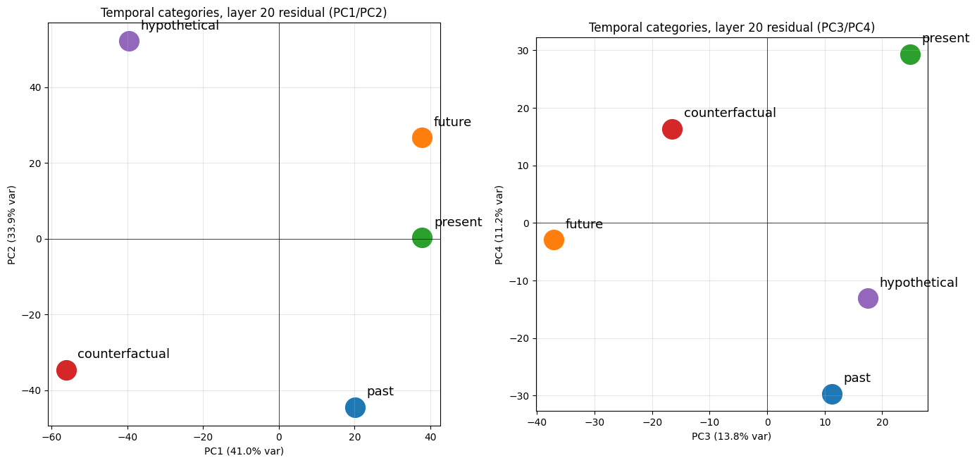
# === STEP 3: Geometry — PCA on category means ===import numpy as npfrom sklearn.decomposition import PCAimport matplotlib.pyplot as pltORDERED_CATS = ["past", "present", "future", "counterfactual", "hypothetical"]# Stack residual stream means → (5, d_model)M = torch.stack([category_means_resid[c] for c in ORDERED_CATS]).cpu().numpy()# Center (recommended for PCA)M_centered = M - M.mean(0, keepdims=True)pca = PCA(n_components=4)M_pca = pca.fit_transform(M_centered)# Plot PC1/PC2fig, axes = plt.subplots(1, 2, figsize=(14, 7))colors = ["#1f77b4", "#2ca02c", "#ff7f0e", "#d62728", "#9467bd"]for ax_idx, (px, py) in enumerate([(0, 1), (2, 3)]):    ax = axes[ax_idx]    for i, cat in enumerate(ORDERED_CATS):        ax.scatter(M_pca[i, px], M_pca[i, py], s=400, c=colors[i], label=cat)        ax.annotate(cat, (M_pca[i, px], M_pca[i, py]),                    fontsize=13, xytext=(12, 12), textcoords="offset points")    ax.set_xlabel(f"PC{px+1} ({pca.explained_variance_ratio_[px]:.1%} var)")    ax.set_ylabel(f"PC{py+1} ({pca.explained_variance_ratio_[py]:.1%} var)")    ax.set_title(f"Temporal categories, layer 20 residual (PC{px+1}/PC{py+1})")    ax.set_aspect("equal")    ax.grid(alpha=0.3)    ax.axhline(0, color="k", lw=0.5)    ax.axvline(0, color="k", lw=0.5)plt.tight_layout()plt.show()print(f"Variance explained: {pca.explained_variance_ratio_}")print(f"Cumulative:         {np.cumsum(pca.explained_variance_ratio_)}")

Variance explained: [0.4102727  0.33915818 0.13833533 0.11223382]
Cumulative:         [0.4102727  0.7494309  0.88776624 1.        ]

Pre-prompt scatter

In [13]:
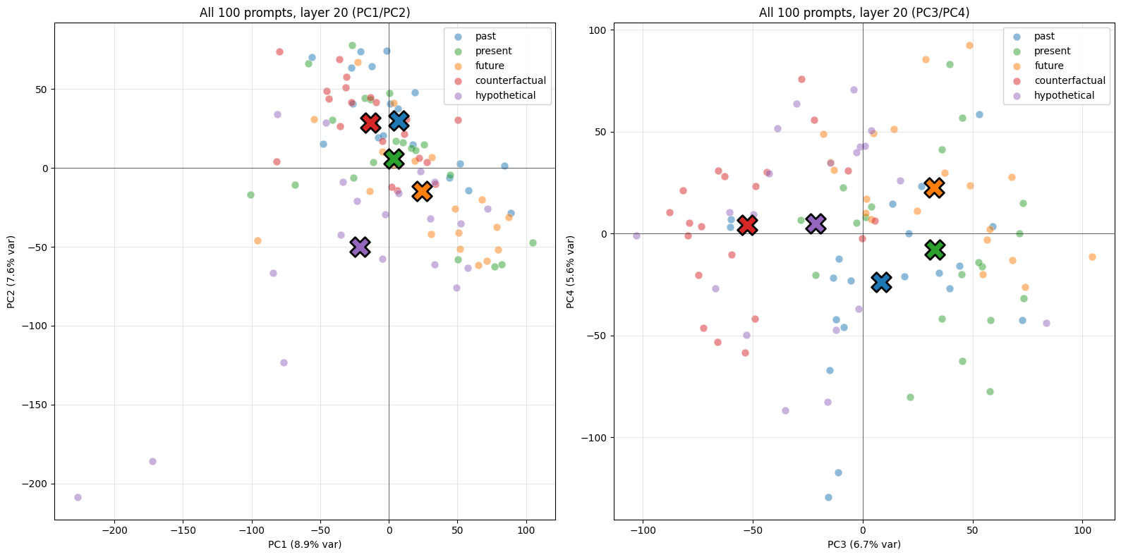
import numpy as npfrom sklearn.decomposition import PCAfrom sklearn.metrics import silhouette_scoreimport matplotlib.pyplot as pltORDERED_CATS = ["past", "present", "future", "counterfactual", "hypothetical"]colors = ["#1f77b4", "#2ca02c", "#ff7f0e", "#d62728", "#9467bd"]# Collect all 100 prompts' last-token residuals at layer 20all_vecs, all_labels = [], []for cat in ORDERED_CATS:    for p in ALL_TEMPORAL_CATEGORIES[cat]:        tokens = model.to_tokens(p)        _, cache = model.run_with_cache(            tokens, names_filter="blocks.20.hook_resid_post", return_type=None,        )        all_vecs.append(cache["blocks.20.hook_resid_post"][0, -1].float())        all_labels.append(cat)    print(f"{cat}: done")X = torch.stack(all_vecs).cpu().numpy()X_centered = X - X.mean(0, keepdims=True)pca = PCA(n_components=4)P = pca.fit_transform(X_centered)# Plotfig, axes = plt.subplots(1, 2, figsize=(16, 8))for ax_idx, (px, py) in enumerate([(0, 1), (2, 3)]):    ax = axes[ax_idx]    for i, cat in enumerate(ORDERED_CATS):        mask = np.array([l == cat for l in all_labels])        # Individual points        ax.scatter(P[mask, px], P[mask, py], s=60, c=colors[i],                   alpha=0.5, label=cat, edgecolors="white", linewidth=0.5)        # Centroid as black-bordered X        cx, cy = P[mask, px].mean(), P[mask, py].mean()        ax.scatter(cx, cy, s=400, c=colors[i], edgecolors="black",                   linewidth=2, marker="X", zorder=5)    ax.set_xlabel(f"PC{px+1} ({pca.explained_variance_ratio_[px]:.1%} var)")    ax.set_ylabel(f"PC{py+1} ({pca.explained_variance_ratio_[py]:.1%} var)")    ax.set_title(f"All 100 prompts, layer 20 (PC{px+1}/PC{py+1})")    ax.legend(loc="best", framealpha=0.9)    ax.grid(alpha=0.3)    ax.axhline(0, color="k", lw=0.4); ax.axvline(0, color="k", lw=0.4)plt.tight_layout()plt.show()# Cluster separation metricslabel_ids = np.array([ORDERED_CATS.index(l) for l in all_labels])sil_2d = silhouette_score(P[:, :2], label_ids)sil_4d = silhouette_score(P[:, :4], label_ids)print(f"\nSilhouette score in PC1-2: {sil_2d:.3f}")print(f"Silhouette score in PC1-4: {sil_4d:.3f}")print("Interpretation: > 0.25 = clear cluster structure, "      "0.1-0.25 = weak structure, < 0.1 = mostly overlapping")
past: done
present: done
future: done
counterfactual: done
hypothetical: done


Silhouette score in PC1-2: -0.119
Silhouette score in PC1-4: 0.010
Interpretation: > 0.25 = clear cluster structure, 0.1-0.25 = weak structure, < 0.1 = mostly overlapping
In [14]:
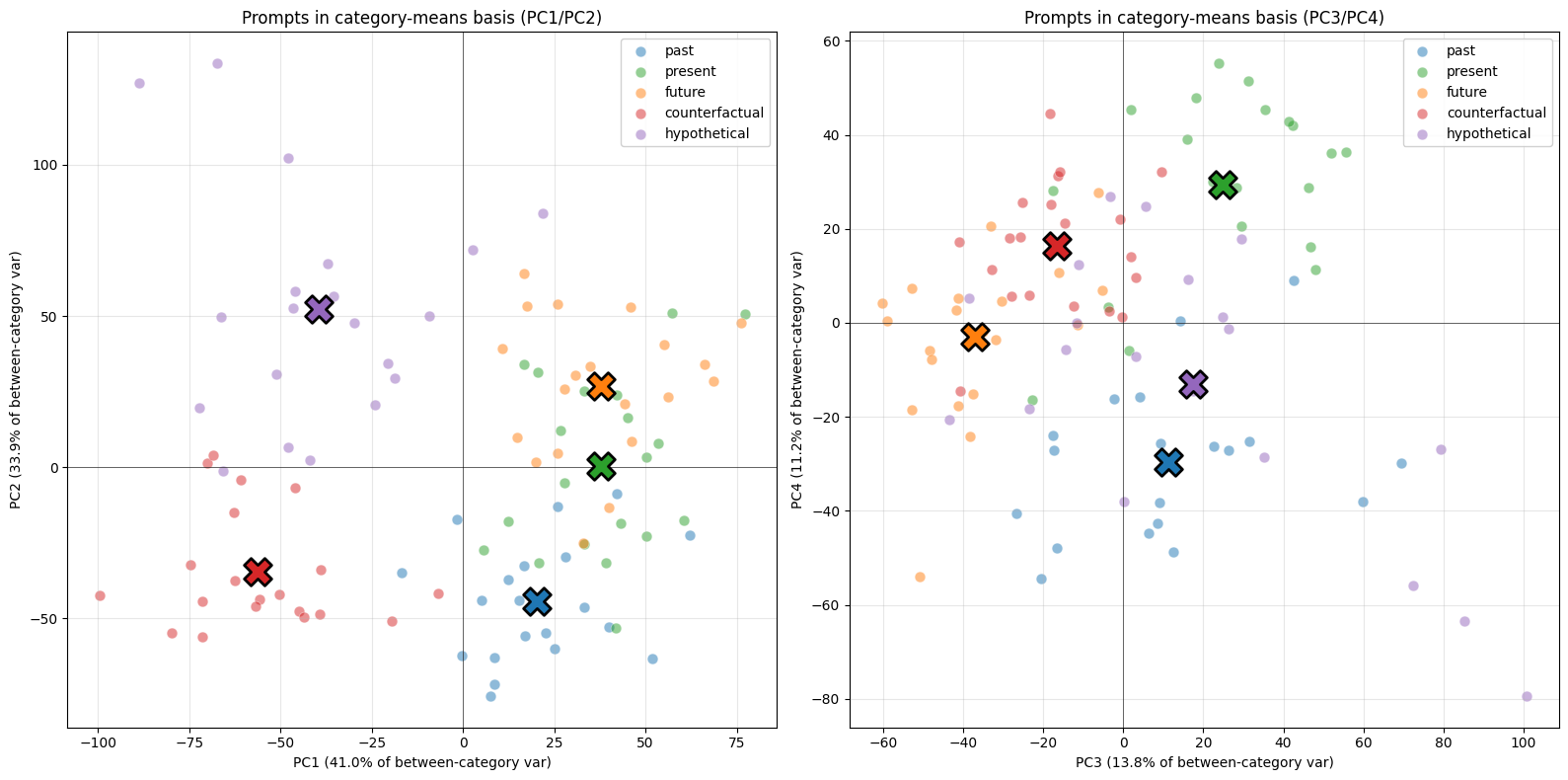
# PCA basis from category means; project individual prompts into itcat_means_raw = np.stack([    X[np.array(all_labels) == cat].mean(0)    for cat in ORDERED_CATS])# Center on grand mean of category meansgrand_mean = cat_means_raw.mean(0, keepdims=True)pca_means = PCA(n_components=4)pca_means.fit(cat_means_raw - grand_mean)# Project individual prompts into the same basisP_mb = pca_means.transform(X - grand_mean)# Plotfig, axes = plt.subplots(1, 2, figsize=(16, 8))for ax_idx, (px, py) in enumerate([(0, 1), (2, 3)]):    ax = axes[ax_idx]    for i, cat in enumerate(ORDERED_CATS):        mask = np.array([l == cat for l in all_labels])        ax.scatter(P_mb[mask, px], P_mb[mask, py], s=60, c=colors[i],                   alpha=0.5, label=cat, edgecolors="white", linewidth=0.5)        cx, cy = P_mb[mask, px].mean(), P_mb[mask, py].mean()        ax.scatter(cx, cy, s=400, c=colors[i], edgecolors="black",                   linewidth=2, marker="X", zorder=5)    ax.set_xlabel(f"PC{px+1} ({pca_means.explained_variance_ratio_[px]:.1%} of between-category var)")    ax.set_ylabel(f"PC{py+1} ({pca_means.explained_variance_ratio_[py]:.1%} of between-category var)")    ax.set_title(f"Prompts in category-means basis (PC{px+1}/PC{py+1})")    ax.legend(loc="best", framealpha=0.9)    ax.grid(alpha=0.3)    ax.axhline(0, color="k", lw=0.4); ax.axvline(0, color="k", lw=0.4)plt.tight_layout()plt.show()sil_mb = silhouette_score(P_mb[:, :2], label_ids)print(f"Silhouette in means-basis (PC1-2): {sil_mb:.3f}")print(f"Silhouette in means-basis (PC1-4): {silhouette_score(P_mb[:, :4], label_ids):.3f}")

Silhouette in means-basis (PC1-2): 0.196
Silhouette in means-basis (PC1-4): 0.310
In [13]: